Calibration process (4 Steps)

Calibration is the process of configuring cameras (or other inputs) to measure crowd movement and distances. You will need to calibrate each camera separately, to map out the space under observation.

Calibration ensures that DCM can supply accurate information to you via the dashboard or any notification. Without detailed information on your cameras and their location, the results presented by DCM will not be accurate as DCM leverages the calibration information to understand the area, distances and positioning of people observed.

Before starting the calibration, the user should identify and consider what areas on the camera view will be measured. Please note that if your environment is complex, such as multi levelled, ramps, inclined planes or has a very large area under observation, you may need to only calibrate a part of it, and consider using extra cameras.

The camera calibration process gets the user to place 'pins' to identify landmarks both in an overhead map view (called the ‘device location view’) and an isometric view of the area as captured by the camera itself (called the ‘device view’). Our software then matches up this information to generate a three-dimensional representation of the area, to calculate crowd position and movement within the space.

In addition to this guide - an online tutorial for the calibration process is available here:
Calibration Tutorial

Depending if the camera to be calibrated is indoor or outdoor, and what landmarks are visible in the view, the process can use either overhead satellite images, user supplied blueprints, objects placed in the camera view or a grid overlay to assist matching up the two views.

In most cases it is not necessary to have someone on site at the camera location, but it can be useful, if practical. This person could place temporary objects such as cones in the view to assist pin placement. DCM can also provide custom calibration sheets that look like a chess board, with one meter by one meter squares to use for calibrations where the site is accessible.

Step 1 : Give a name to the calibration

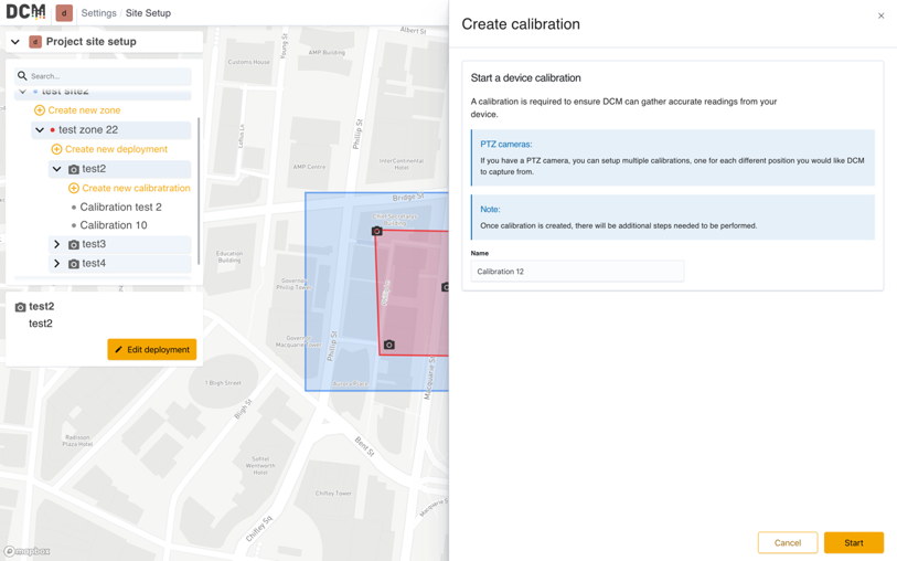
Enter a calibration name and press ‘Start’

This will present a new screen where you will load a ‘Device location’ (an overhead map, grid or plan) and a ‘Device view’ (captured from the camera), and map landmarks between them.  Load both views using the yellow buttons before starting to place pins.  If either view fails to load, consult the troubleshooting guide at the end of this section.

Step 2: Calibrate device location

Sample Calibration screen before loading device location and device view.

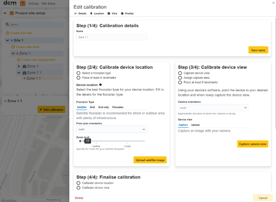
The device location section (left side of the screen) identifies the area under capture in an overhead view.  Depending on the environment (for example indoor or outdoor) there are four visual guide options available to help you.

Satellite:

Is good for outdoor, open areas with plenty of infrastructure that can be identified on the satellite map and on the camera view. For example on a street with permanent landmarks and features around it.

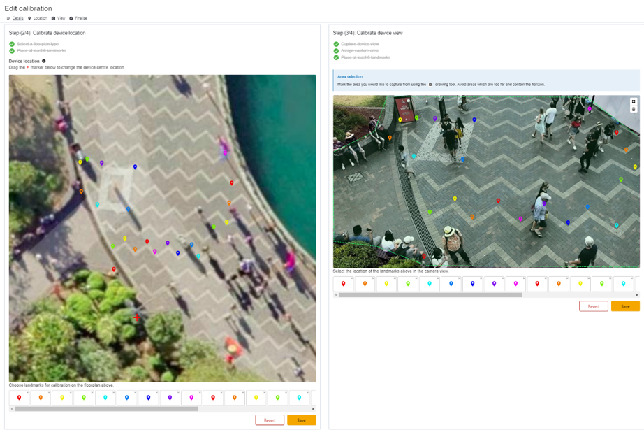
If the user selects Satellite, your main guide will be an overhead view of objects already in the cameras view zone. Choose at least six landmarks on the map to mark.  and place marker pins by left clicking on the map.   The first six marker pins are mandatory.  select or add markers from the menu below the map view.  To place a marker pin, left click on a pin icon, then left click on the map to place it.  A landmark is an object displayed in the view that has a fixed location and easy to be found on the map.

A completed outdoor calibration, using satellite mode, with regular patterns on the ground used as key calibration points.

Grid:

The most versatile and generally recommended option.  This option still uses the satellite view, but overlays it with a grid of a defined size, so gives you most of the advantages of both.  The only disadvantage is that some objects on the satellite image can be slightly harder to see due to the overlay. This option is best if you know the measurements of some objects in the scene and need to use them to estimate other distances, or if you intend to combine permanent landmarks with temporary markers such as cones to calibrate.  The grid overlay gives you extra information when the area has few permanent physical features easily identified in overhead view, such as a park, road  or other open area.  .

Grid only:
Similar to the grid method but with this option you will get a blank grid without the satellite view in the background.  This option is best for situations where neither an outdoor satellite view, or indoor floorplan is available, but requires the most effort.  You will be entirely reliant on physically measuring the distance from the camera to temporary markers in the camera view.        

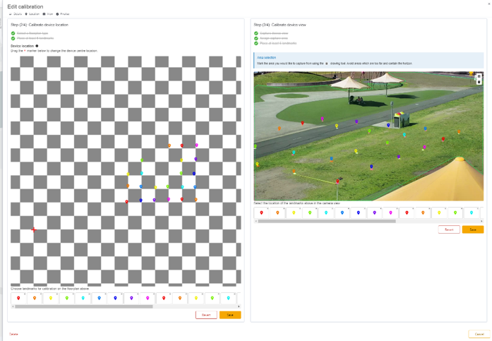
For either Grid or Grid only options, you will need to setup the size of the grid and press ‘upload grid’ to generate a map.   To create landmarks in Grid method, the user will need to physically place some markers on the location, usually in a square grid pattern. Each marker on site will need to have equal distance. User will also need to measure the distance and orientation between the closest marker and the camera at ground level.          

The grid options also have an input to rotate the grid by a given amount, entered as degrees from due north. You may need to load the grid several times to align it optimally with your cameras view, so make sure you are satisfied with both views before placing pins. Reloading the views with clear previously placed pins.

A completed calibration in grid only mode, using temporary cones as calibration points.       

Floorplan:
If a floorplan with reliable measurements is already available for an indoor area, such as a conference hall or an exhibition centre, using this option will reduce the need for physical measurements. 

Select upload Floorplan to upload your file and generate a guide view.  Then apply the same process to mark the landmarks.           

A marker can be anything that is visible in the camera view.  This may be a permanent landmark, but also can be a temporarily placed one such as a cone or flag.
it is recommended that markers are at least six meters from the camera for best results. 
The more markers you can place, the more accurate the final calibration will be.  The minimum is six, but a dozen or more is better.              

Step 3 Calibrate device view

Press the button to capture a view from the camera. If this fails, consult the troubleshooting guide at the end of this section.  Do this after placing any temporary markers and before placing any pins on either view.  Ensure the camera is aligned optimally to view the area of interest, using its native VMS if necessary. The view as captured should include all landmarks from the overhead map that you plan to use.     

Here the user will draw the area to be used for analysis, referred to as the ‘foot level mask area’, and then place pins to indicate the position of the same landmarks used for the overhead view.

The drawing tool works similarly to the previous version used to map out Sites and Zones.
Try to define only ground or floor level areas.  Any area outside this boundary will be effectively ‘masked’ and will not be used by DCM.  Although people partly in the defined area will still be counted.  This can be useful, especially if you have cameras with overlapping views.

Keeping the shape as simple as possible, will reduce the chance of error in the final results. Avoid defining the bottom part of walls or the horizon in your area.  It is generally better to draw the area just inside natural boundaries leaving a small gap.  This is especially true at the far end of the view.  Because of the effect of perspective,  even overestimating by a few pixels can heavily affect the calibration, resulting in inaccurate density results.

Place pins in a consistent manner, where the landmark meets the floor or ground level.  Landmarks toward the centre of the view work best for small sample areas under 100 meters square.  For wider views, especially if the camera has significant ‘fish-eye’ visual distortion, calibration accuracy can be improved by supplementing with a few wider points toward the edges if possible. Consider augmenting permanent landmarks with temporary ones such as cones or bollards.  When using temporary landmarks, arranging them in a grid or regular pattern will generally get the best results.  Measure the distance from your camera to your landmark and confirm it matches the expected location using the grid or plan.

You can zoom in and out of both views using the mouse wheel or on screen controls to aid with pin placement.   

When you first draw the foot level mask area, the device view will show the polygon you have created as a dashed green line,  but will also add a second polygon area slightly above it.  This is the ‘head level mask area’.  Initially it will be created automatically a short distance above your drawn foot level polygon.

The reason there are two masks is because DCM has two available detection modes,  ‘Pedestrian Detector’ (PD) and ‘Head Detector’ (HD) modes.

When in the default ‘PD’ mode – all people at least partly within your drawn ‘foot level mask’  will be included in the statistics.  If you swap to HD mode, the system will count heads that fall at least partially within the upper mask.
With pins placed on the overhead map or grid,  matching pins on the camera view,  and a foot level mask area drawn your calibration should look something like this.

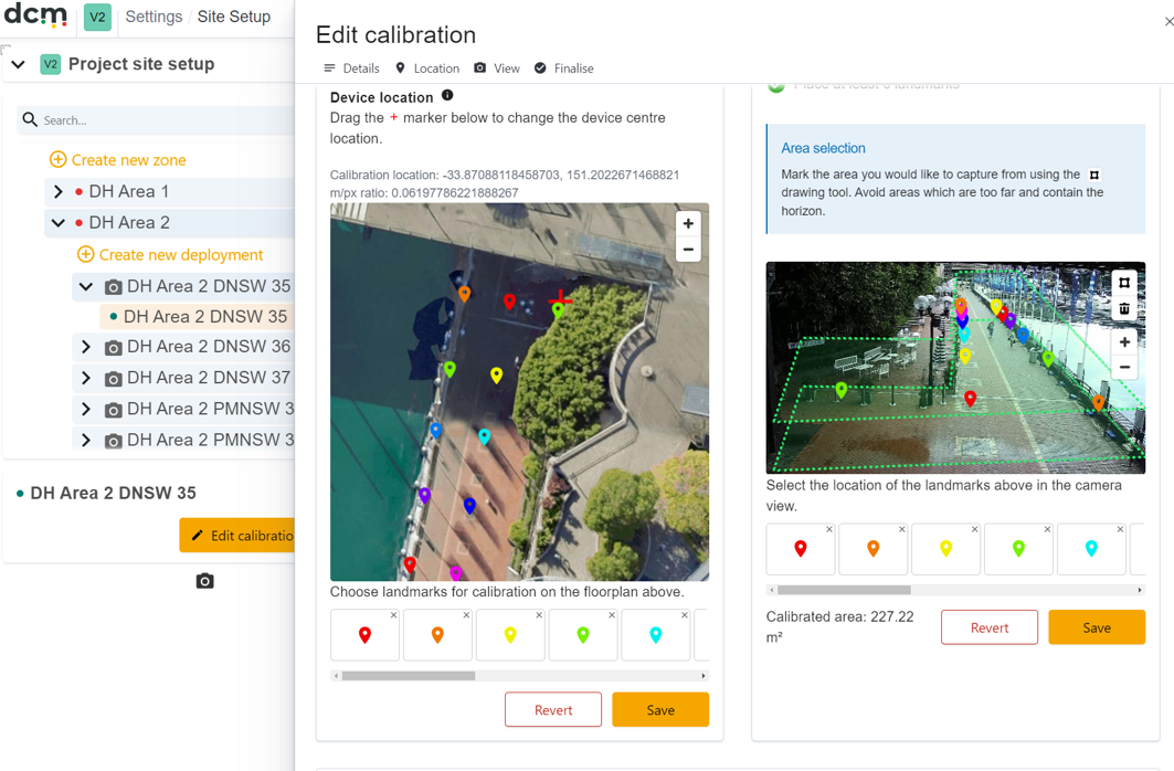
Depending on the height and orientation of the camera, it is likely you will need to adjust the default position of the ‘Head level mask’ to more accurately reflect where peoples heads will be.
Most likely you will need to lower the head level mask for positions further away from the camera to account for perspective from the camera viewpoint.  Point in the top mask should remain vertically in line with points in the foot level mask to ensure that both masks count people in the same area.
Defining simple mask shapes, such as a simple four sided rectangle in the center of the view will make this process easier, and reduce potential for error.

The mask position can be adjusted by selecting a point on the polygon with your mouse, holding down the mouse button and dragging the point to the desired position.

For the above example,  even the points near the front are a little too high for even the tallest person,  and the level at the back should be adjusted down the most.  Objects in the view can assist with height estimates.  If possible it is helpful to take your calibration image with at least one person in your desired mask area to assist with this adjustment.

For cameras that are at a high angle, you may need to adjust the rear mask down quite significantly.
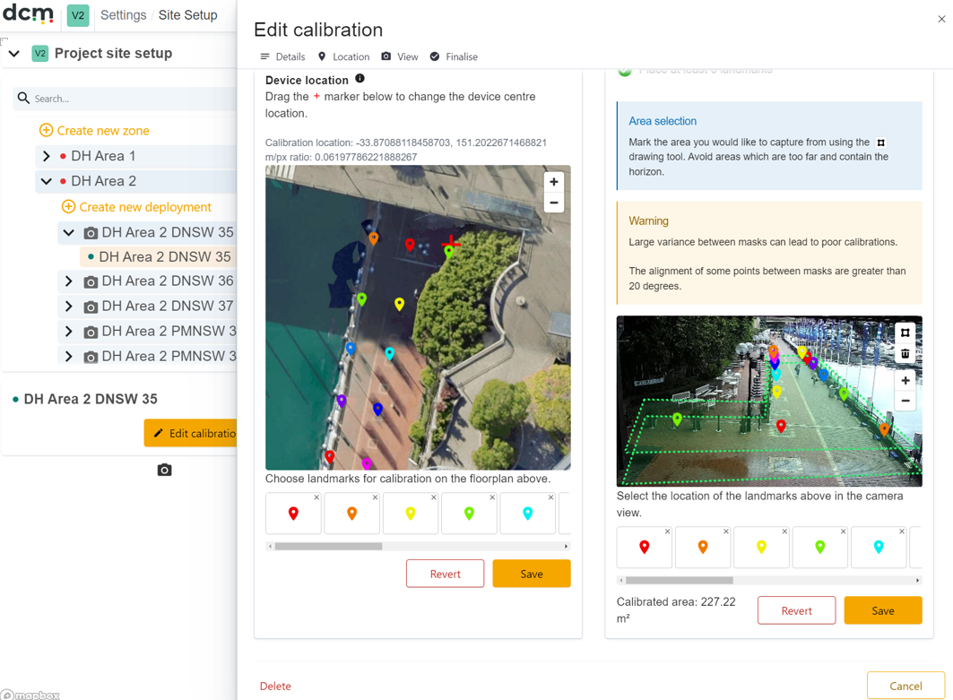
You may see a warning appear that the angle of the head and foot masks varies by more than 20 degrees.  For many views, this is normal, and this warning can be safely ignored.

With all landmarks placed in both windows, the foot mask drawn,  and the head mask adjusted to fit the view, your finished calibration will look something like this.   

📌 Pin Placement Tips

In general Pins do not have to be placed within your intended mask, but are more useful for calibration accuracy if they are. Pins placed exactly on the boundary line, and especially in the corners of your defined area can be problematic, and are best avoided if possible.

💡 General Guidelines

• For smaller view areas, roughly under 100 meters square a regular central grid of pins tends to work best, and give best calibration accuracy.

• For wider views supplementing central points with a few closer to the edge can be beneficial, especially if camera has fish-eye distortion or is relatively low.

• Avoid placing points at the edges of the view area, especially in the far distance if possible, especially if camera angle is low.

• Keep points on a single plane. This doesn’t have to be flat, but does need to be consistent.

Step 4: Finalise the Calibration             

Press ‘Start calibration’.  At this point the software will match up the pin positions between the camera view, and the satellite or grid view and generate a calibration.    

If this fails, or the results seem inaccurate, consult the troubleshooting guide at the end of this section.

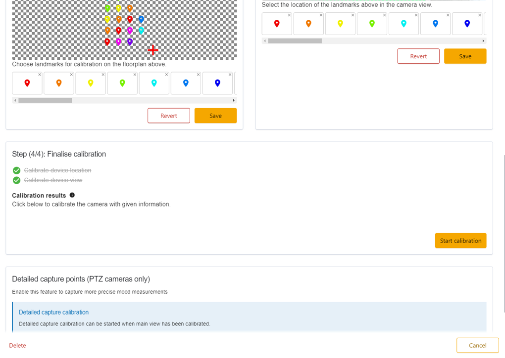
 If the Calibration is successful, the calibration results section will appear.

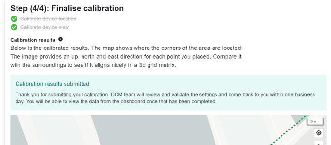
This consists of two sections – a map showing an example heatmap, marking out the area you defined.  And a new camera view with guide arrows as below.

The sample heatmap should have points in a relatively compact pattern that covers the expected area of the map, and does not ‘spray’ any greet heatmap sample points over a wider area of the map.

In the new camera view, there will be two lines on each landmark. The green lines should point to North and the Red lines should point to East. Each line should represent one metre.   If the result does not look similar to the example below, it may indicate an issue with data input or pin placement.   You may need to redo the process in step 2 and step 3.

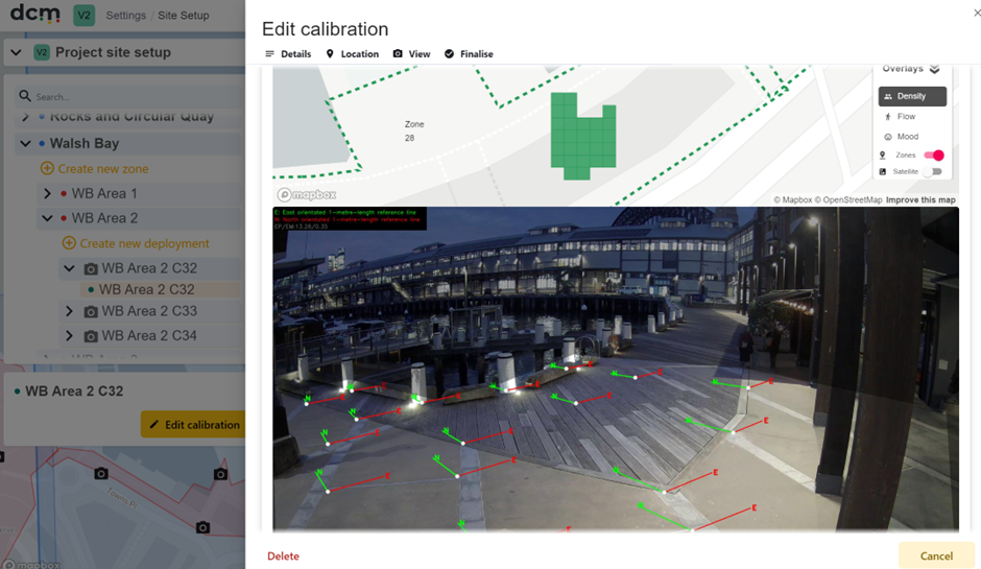
Checking for accuracy and correcting issues  

There are some additional visual aids to check the accuracy of the calibration.  Each North/East line pair is linked by a round circle.  These circles are coloured either white, orange of red.  When calibrating, the software tries to determine map the surface.  This is much more accurate if calibration points are on a single plane.  Points coloured red, are outliers compared to the overall calculated surface.  Orange points are marginal.     
In general these are good candidates to be re-positioned or deleted.   They may not necessarily be ‘wrong’ or inaccurately placed, but they are outliers when compared to the bulk of other points. 

There is also a numerical indicator of overall calibration accuracy. 
In the top left of the calibration image, there is a line that reads “EP/EM” followed by two numbers.
This is the calculated error per pixel and error per meter.  The per meter number is the most useful for calibration assessment.  As a general rule, error per meter should be kept at 0.6 or less for good accuracy.  If this number is over two, then the scale is likely to be severely over estimated, and calculated distances between people may be very inaccurate.            

In this example, the Error estimate is highlighted within the red box.  And a problem area in the calibration, with both red and orange ‘dots’ is highlighted within the blue box.     

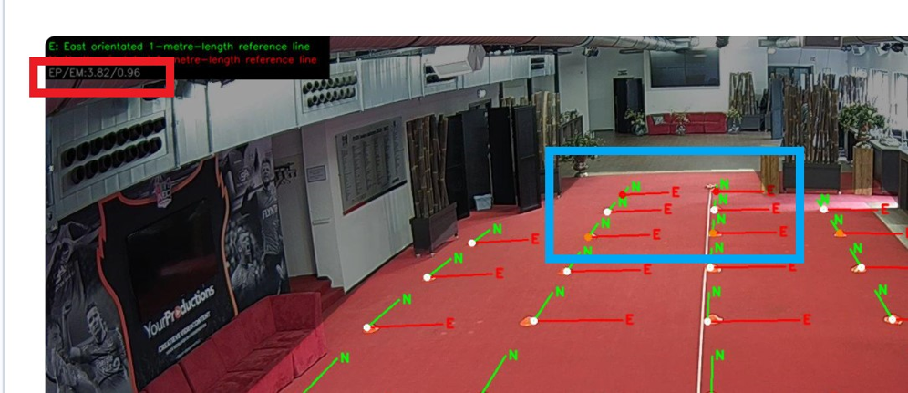
In this case, the two furthest points are likely to be inaccurate due to distance and fish-eye distortion from the camera lens.  Accuracy could be improved from the current 0.96 value by simply deleting them.

The most important indicator of calibration accuracy however, is the sample map on the calibration screen, visible once a calibration has been successfully submitted.

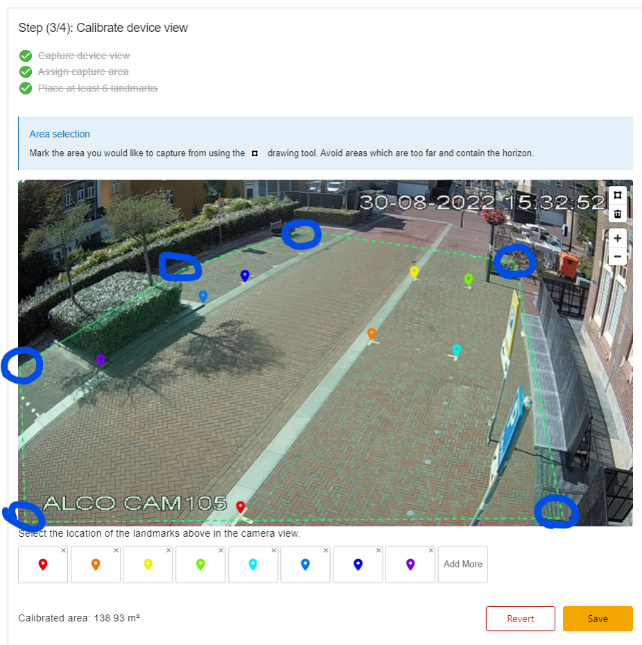
(Above) A sample calibration input with a six sided polygon calibration area defined.  Corner points are highlighted in blue.  After the calibration is submitted, the calibration engine returns the camera view and guide lines, and also a map, simulating a person standing at each polygon ‘corner’ (Below).  Even though some of the North/East arrow indicators are distorted due to being near the edge of the view, the position of the sample detections are in the correct locations.  This is the strongest indicator that the final latitude/longitude positionings will be correct, and indicates a good calibration, despite a low number of points used, and the distorted appearance of some indicator arrows.            

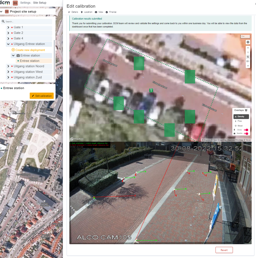
To re-do the calibration, press the “Revert”  button below the image.  Then make your adjustments to the pins in the device view and/or device location.  Once complete – press  “Start Calibration” again.

If this does not rectify the issue, you can consult the troubleshooting guide in the next section.
If you still cannot obtain a calibration that seems acceptable, contact DCM support.

💡 Calibration Accuracy Assessment Advice

To summarise the advice on assessment of calibration accuracy:

✔ Accurate Calibration Checklist (Decreasing Order of Importance)